Fixed Strike Volatility, Floating Strike Volatility, Spot Vol Dynamics And The Skew Stickiness Ratio Part 1

04 Jul 2026

Intro

Today I want to talk about some topics in the volatility space that confused me for a long time but are extremely important to understanding volatility modeling and volatility trading nomenclature. The terms fixed strike volatility, floating strike volatility, sticky strike and sticky delta come up a lot and are sometimes thrown around loosely. On top of that, if we add fixed strike skew and floating strike skew into the mix, the terminology becomes even more confusing. Sometimes skew is even replaced with spot-vol beta, covariance, correlation, and many other related quantities. It is easy to see how these definitions can become confusing. I’ve seen many well established successful people in the vol space use these definitions in different ways and that is part of the reason why they can be so confusing. I Specifically hear people use sticky strike and fixed strike interchangeably even though they are different concepts. What I want to do in this post is talk about how I like to think of them and give some examples of their usage in the world of volatility.

Definitions

I am going to start off by simply defining these terms and maybe giving you a few pictures to hammer home the meanings. A great way to think about these which was eloquently defined by Benn Eifert from QVR is “Sticky strike and sticky delta refer to spot vol dynamics and fixed strike and floating strike vol are specific parameters of the volatility surface”. Not sure if this is an exact quote but close enough. That definition is something you should keep in your head especially as we move forward throughout this post (and in future posts) and I will often go back to it.

Fixed Strike - Floating Strike Volatility

What does it mean to parameterize a volatility surface, well in mathematical terms we can represent the volatility surface as some function $\sigma(.)$ that has specific parameters that when we plug them in we get an implied volatility. On a fixed strike basis the parameters would be strike K and maturity T $\sigma(K, T)$. In general I like to think about the parameterization of the volatility surface as how we define the x-axis, for fixed strike we use our strikes and for floating strike it would be something like delta $\sigma(\Delta, T)$ or moneyness $\sigma(k, T)$ ($k = K / F$). How we define our parameterizations becomes especially important in stochastic volatility modeling where using either a fixed or floating strike parameterization will change the dynamics of our implied volatility process, ATMF instantaneous skew, SSR and P&L dynamics.

What really helped me understand these concepts was reading through Emanuel Derman’s volatility lectures. In those lectures, he explains the difference between fixed strike and floating strike volatility from a time-series perspective, and I think this visualization makes the distinction much clearer. Below, I plot the time series of several fixed strike implied volatilities. At the starting date, I select options with specific strikes and then track the implied volatility of those same strike options over time. In this example, we begin on 2026-01-01 with the underlying trading at 680 and choose strikes ranging from 660 to 700. As time passes the underlying price changes but each series always represents the implied volatility of the option with it’s original fixed strike. For example, the series labeled 660 is simply the implied volatility of the K=660 option on every subsequent trading day.

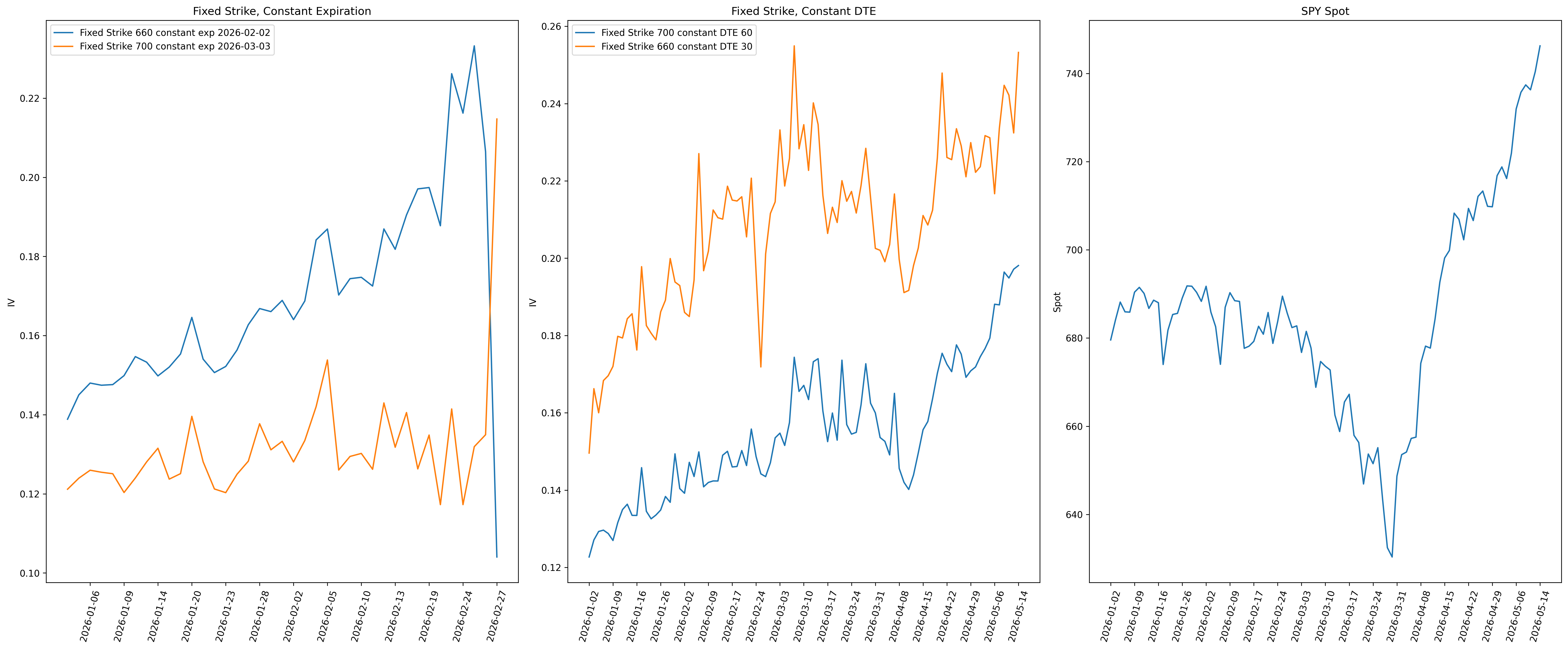
It is also important to distinguish between constant expiration and constant maturity, just as we distinguish between fixed and floating strike. The charts above illustrate both approaches. Under a fixed strike vol constant expiration framework, the expiration date remains fixed throughout the time series, meaning we follow the same option contract every day. As time passes, the contract loses one day of maturity at each observation for example, a 30 DTE option on day one becomes the same contract with 29 DTE on day two, then 28 DTE on day three, and so on. In contrast, a fixed strike vol constant maturity framework keeps the days to expiration fixed rather than the expiration date. Generally we observe a different option contract each day, selecting (or more commonly interpolating between) the two expirations that most closely target maturity. This distinction is important when designing backtests and rebalancing trading strategies, as the choice between constant expiration and constant maturity can materially affect the behavior and interpretation of the resulting option prices.

Next we show similar graphs for a floating strike volatility time series. Unlike the fixed strike vol case, the strike is no longer held constant. Instead, we keep the chosen volatility surface parameterization such as moneyness or delta fixed through time. As the underlying price changes, the strike corresponding to that fixed moneyness or delta changes as well. Consequently, every implied volatility in the time series generally refers to a different strike and, therefore, a different option contract.

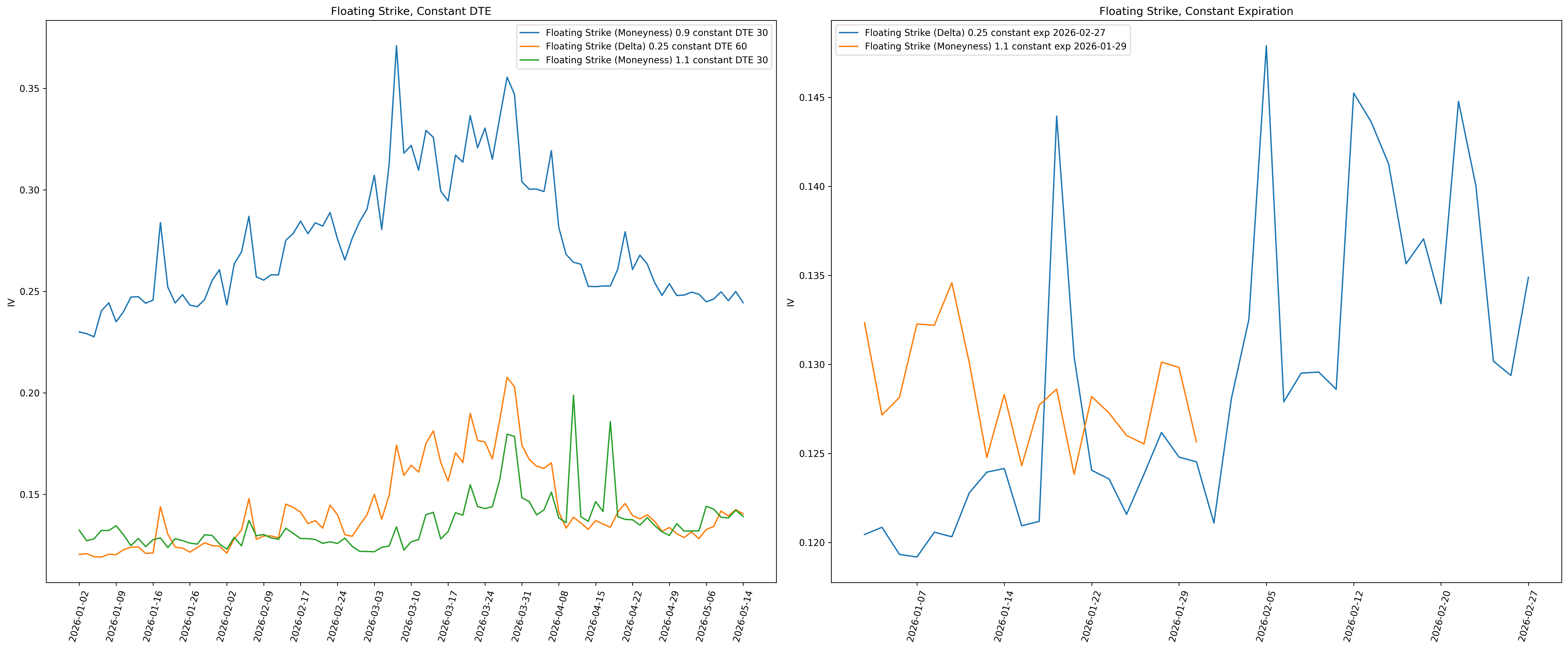
Usually when someone plots a rolling chart of some implied volatility metric it is usually a constant maturity floating strike volatility. For example if you ever see someone post a chart of the ATM IV it is most of the time a constant maturity floating strike ATM IV but nobody ever defines it like that. Another common example is the VIX, while the VIX is technically neither a fixed or floating strike vol, its time series behaves like a constant maturity floating strike vol metric. the distinction between fixed and floating strike IV is hardly made but it is important as the below example illustrates.

If you are trying to trade a pure long volatility position by, let’s say, buying a straddle and delta hedging it, you usually start by buying the ATM put and call. The issue is positions and trades are not floating strike, they have to be discretely rehedged to become semi floating strike. If you buy a delta hedged straddle today and don’t look at it for a week more likely than not the original spot price will have moved away from ATM and it is no longer ATM anymore. On a fixed strike basis how vol changes is hugely important to our positions P&L, did fixed strike follow the skew curve, did the fixed strike vol meaningfully outperform the skew curve. These are all things options traders look at and need to know and will bring us to our next topic but I briefly want to touch on fixed strike and floating strike skew.

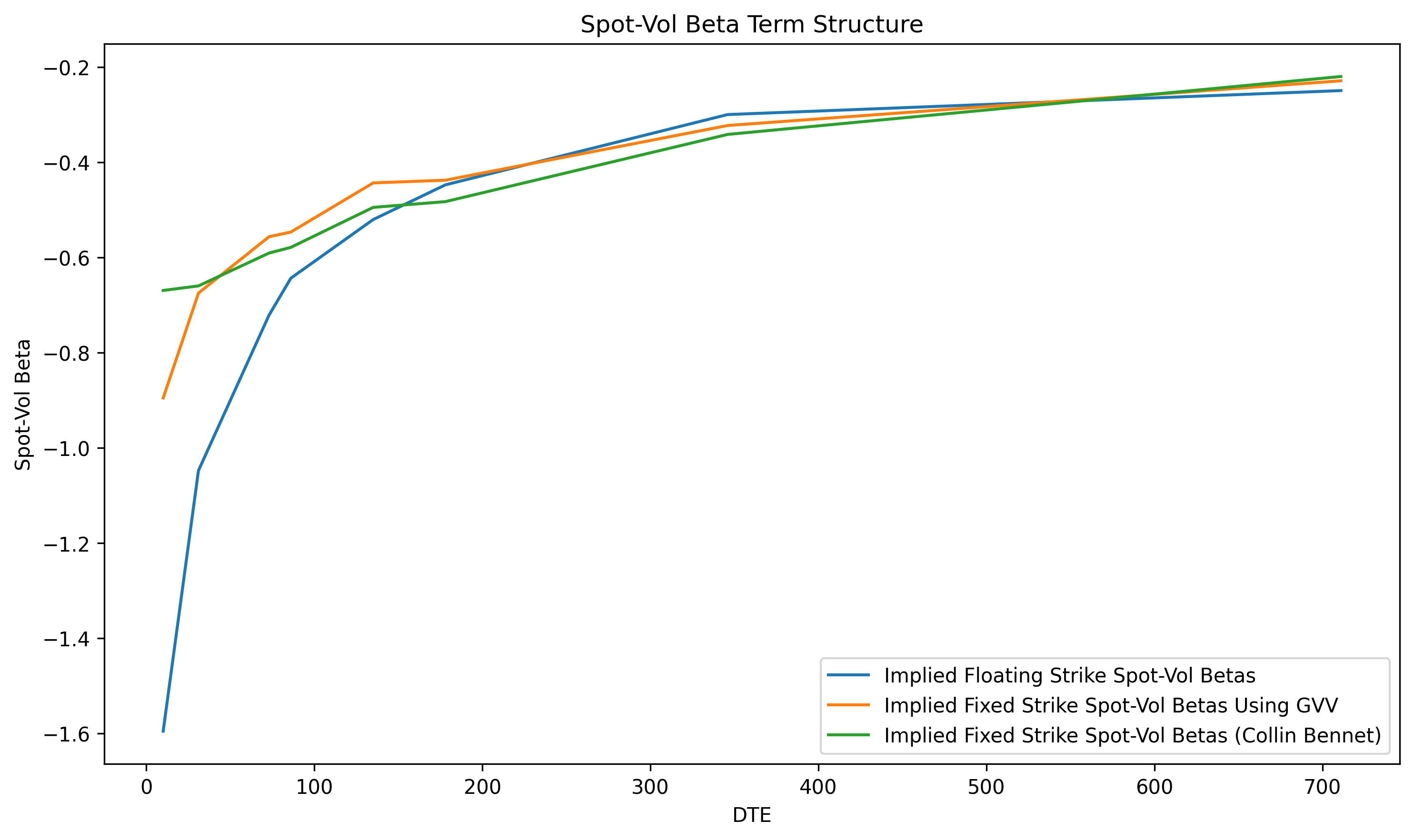
Fixed strike skew and floating strike skew is another concept that confused me for a while. To avoid confusion, it is important to note that these are not the same as the fixed strike and floating strike volatility time series discussed above. Instead, they refer to two different ways of measuring the slope of the implied volatility smile. Fixed strike skew is a volatility independent measure because it is calculated using the same fixed strikes (or moneyness levels) regardless of the level of implied volatility. Floating strike skew is volatility dependent because it is defined using option deltas, and the Black-Scholes delta itself depends on the assumed implied volatility. As volatility changes, the strikes corresponding to a fixed delta also change.

Fixed strike skew = \(\sigma_{90\% moneyness} - \sigma_{110\% moneyness}\)

Floating strike skew = \(\frac{\sigma_{25\Delta\,\mathrm{put}} - \sigma_{25\Delta\,\mathrm{call}}}{\sigma_{50\Delta}}\)

The distinction is best illustrated by examining the skew term structure at a single point in time. In the chart below, the fixed strike skew is computed using the same strikes for every maturity, while the floating strike (delta) skew is computed using the same deltas. Because the strikes associated with a given delta vary across maturities, and depend on the level of implied volatility, the floating strike skew is evaluated using a different set of strikes at each expiration. The difference between these two measures is most noticeable for short dated options, where changes in volatility have a much larger impact on the strike corresponding to a given delta. Although I label these as spot vol beta term structures, they are ultimately measuring the same underlying object.

Spot Vol Dynamics

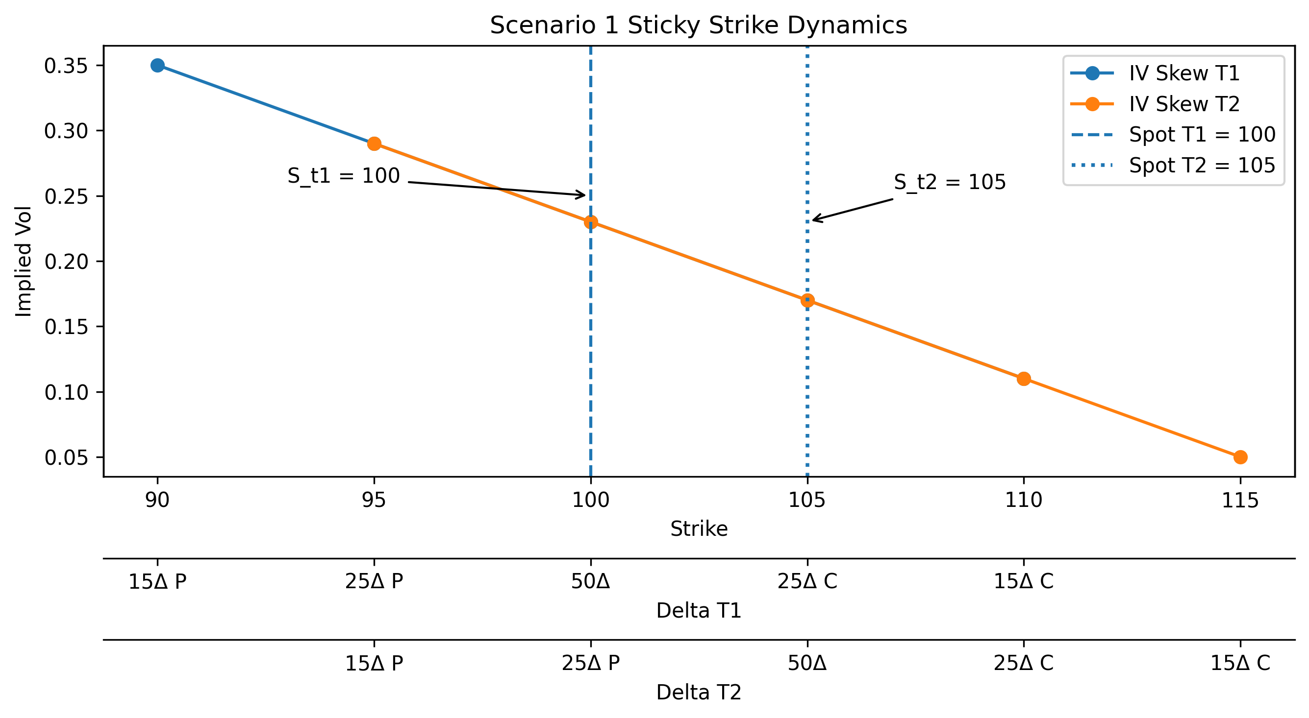
As mentioned above spot vol dynamics are wildly important for volatility trading. The profitability of skew trades like a long (short) delta hedged risk reversal directly depend on the dynamics of the volatility surface. Also the delta we should choose to hedge with depends on how we expect vol to move as spot moves. The two most commonly talked about spot vol dynamic “regimes” are sticky strike and sticky delta. Essentially sticky strike says as spot moves the ATM iv will just float along the skew curve, if yesterday spot was 100 with ATM iv 22 and the 105 strike iv was 21, then tomorrow if spot moves to 105 the ATM iv will be 21. As spot moves iv at every strike stays the same, but the deltas shift. Sticky delta says the ATM vol (actually whole skew curve) remains constant with a floating strike parameterization. As spot moves from 100 to 105, ATM iv stays at 22, essentially the whole skew curve shifts. The IV at each corresponding delta stays the same as spot moves around, this is why its called sticky delta.

It’s important to note that there are other spot vol regimes. For example Colin Bennet defines two more in his book “Trading Volatility”, one being sticky local vol and jumpy vol. Emanuel Derman also describes a regime he calls sticky implied tree which I believe is the same as sticky local vol but I’m not 100% sure. Fundamentally, a spot vol regime is simply an assumption about how the implied volatility surface responds to changes in the underlying spot price. Each regime therefore inherently specifies a different relationship between spot movements and the evolution of fixed-strike vol, floating-strike vol, and the rest of the implied volatility surface.

Parameterization	Sticky Strike Behavior	Sticky Delta Behavior	Sticky Local Vol Behavior
Fixed Strike	Independent of index level	Increases as spot level increases	Increases as spot decreases; decreases as spot increases
Floating Strike	Decreases as spot level increases	Independent of index level	Increases as spot decreases; decreases as spot increases

I want to illustrate below how these regimes will affect a delta hedged short risk reversal, ie long skew. In my examples I will use a linearly inverted skew curve for simplicity, and show how the value of our option positions will change based on a move in spot and a move in the skew curve over a 15 day period. We construct a portfolio \(\Pi\) that is long a 95 strike put and short a 105 strike call and buy delta shares to hedge (short risk reversals have negative delta so we buy stock to hedge). We hold this position for 15 days without adjusting the hedge and calculate the P&L. As will see below in both regimes our position will lose money.

Scenario 1: Sticky Strike Dynamics Delta Hedged Long Skew P&L

Time 1:

$\quad P(S_{t_1}, t_1) = 1.058 \quad C(S_{t_1}, t_1) = 0.678 \qquad \Delta_{t_1} = -0.465$

$\quad \Pi_{t_1} = 100P(S_{t_1},t_1) - 100C(S_{t_1},t_1) + 100\Delta_{t_1}S_{t_1} = 4693$

Time 2:

$\quad P(S_{t_2}, t_2) = 0.058 \quad C(S_{t_2}, t_2) = 2.07$

$\quad \Pi_{t_2} = 100P(S_{t_2},t_2) - 100C(S_{t_2},t_2) + 100\Delta_{t_1}S_{t_2} = 4686$

Final:

\[\boxed{\mathrm{P\&L} = \Pi_{t_2} - \Pi_{t_1} = -6.7}\]

The important thing is that under sticky strike both positions initial IV does not change from $t_1$ to $t_2$ which impacts our ending P&L.

Scenario 2: Sticky Delta Dynamics Delta Hedged Long Skew P&L

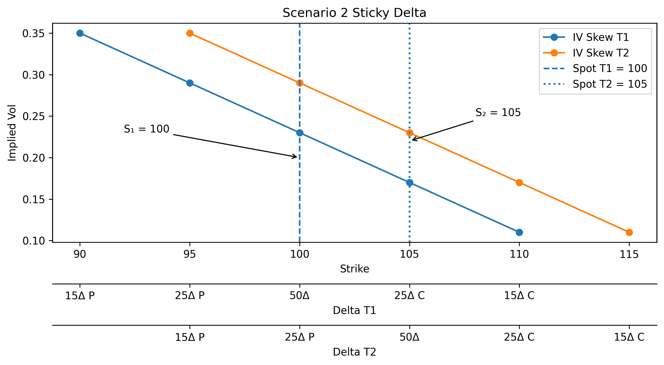
We have the same initial put price, call price and position delta, but because our option positions IV change at $t_2$ we will get different prices.

$\quad P(S_{t_2}, t_2) = 0.13 \qquad C(S_{t_2}, t_2) = 2.73$

$\quad \Pi_{t_2} = 100P(S_{t_2},t_2) - 100C(S_{t_2},t_2) + 100\Delta_{t_1}S_{t_2} = 4627$

\[\boxed{\mathrm{P\&L} = \Pi_{t_2} - \Pi_{t_1} = -66}\]

In this scenario we actually lost more money. Generally for a skew position to be profitable we want the floating strike vol to outperform the fixed strike vol which in this scenario actually happened, so why didn’t our portfolio make money? Well there are a lot of caveats to this but essentially the outperformance of the floating strike call vol overpowered the floating strike put vol.

In this particular scenario where spot moves up we get shorter vega (approaching short call) and suffer more from the call IV rising. For a long skew position to be profitable when spot increases we would ideally like a regime where floating strike vol outperforms fixed strike on the put side, and on the call side fixed strike vol “rolls under” our delta strike vol.

Scenario 3: Sticky Local Volatility Dynamics Delta Hedged Long Skew P&L

Local volatility is another way of modeling vol where we assume the instantaneous volatility is a function of the current asset price and time \(\sigma_{t} = \sigma(S_t, t)\). My favorite definition of local volatility once again comes from Emanuel Derman’s lecture series where he defines local vol as the volatility that justifies current option prices given spot is at a certain level and time in the future.

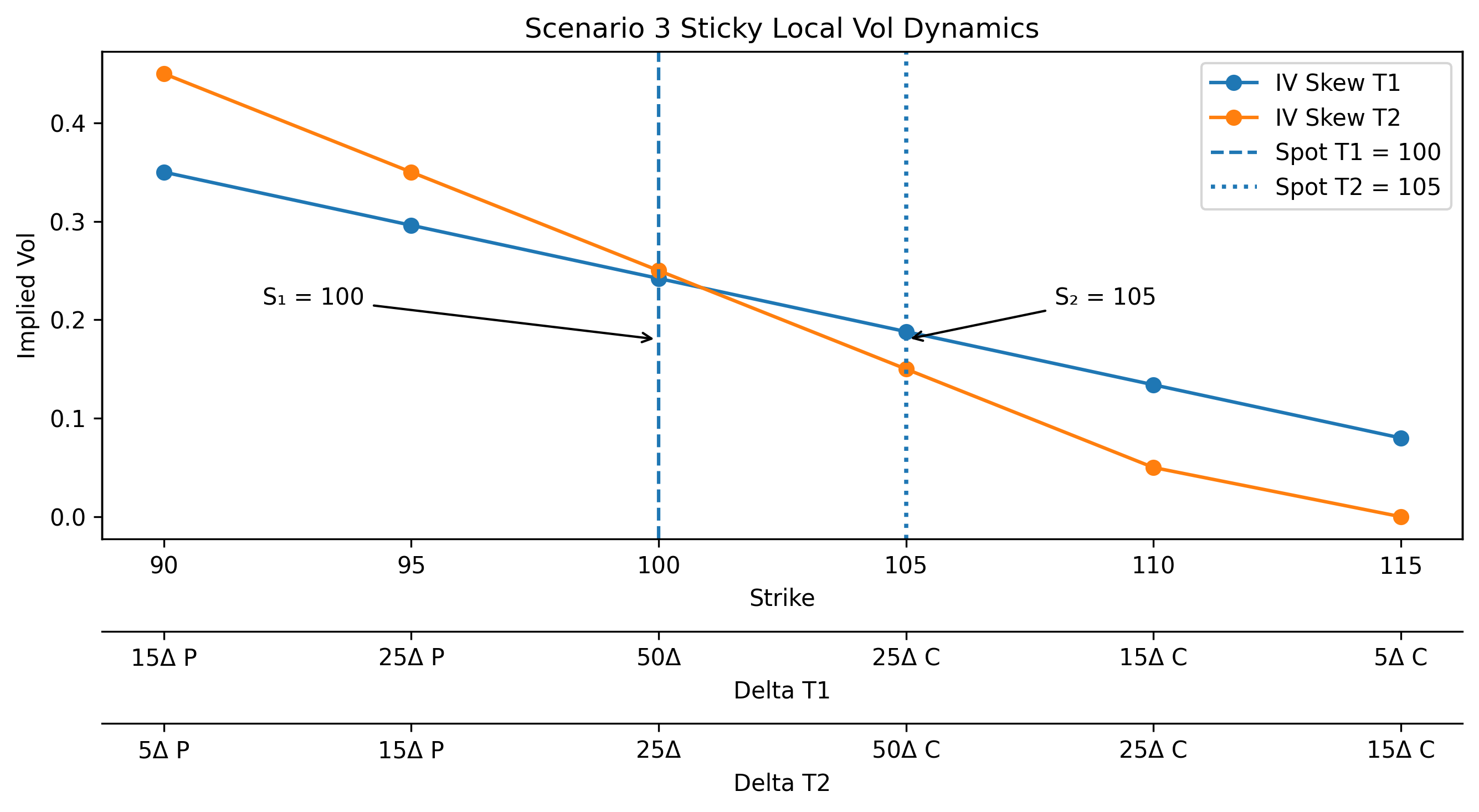
In the sticky local vol regime we assume that ATM IV rises as the market falls, ie negative spot vol correlation. But unlike the other volatility dynamics sticky local vol is not a unique transformation of the smile, as spot moves the exact way the skew rotates depends on the calibrated local volatility surface. Below we show a skew shift that would be advantageous to our Long skew position.

Time 1:

$\quad P(S_{t_1}, t_1) = 1.147 \qquad C(S_{t_1}, t_1) = 1.04 \qquad \Delta = -.5$

$\quad \Pi_{t_1} = 100P(S_{t_1},t_1) - 100C(S_{t_1},t_1) + 100\Delta_{t_1}S_{t_1} = 5200$

Time 2:

$\quad P(S_{t_2}, t_2) = 0.12 \qquad C(S_{t_2}, t_2) = 2.15$

$\quad \Pi_{t_2} = 100P(S_{t_2},t_2) - 100C(S_{t_2},t_2) + 100\Delta_{t_1}S_{t_2} = 5247$

\[\boxed{\mathrm{P\&L} = \Pi_{t_2} - \Pi_{t_1} = 47}\]

You can see in this regime dynamic we actually make money on the long skew trade.

A Note on Deltas

In each scenario I used a basic Black Scholes delta, in reality when you are trading skew you would want to use a “skew delta” which essentially adjusts our delta for how vol will move when spot moves. The Black–Scholes delta is the correct hedge only if implied volatility does not change when spot moves. For equities this will give us a lower delta than BS because we assume a negative spot vol correlation. Once you assume smile dynamics, the hedge becomes:

\[\Delta = \Delta_{BS} + \text{Vega}\,\frac{\partial \sigma_{\mathrm{imp}}(S,K,T)}{\partial S}\]

Each spot vol regime implies a different relationship between changes in the underlying asset and changes in implied volatility. As a result, there is no single “correct” skew delta. Instead, skew delta is model-dependent, and different models produce different corrections to the standard Black-Scholes delta. The appropriate choice often depends on the asset class and market being traded. For example, the Bartlett delta is widely regarded as the market standard for interest rate options because it accounts for the smile dynamics observed under the SABR model.

How important are the simple sticky-strike and sticky-delta assumptions in practice? To quote Benn Eifert once again, it is probably best to forget that sticky strike and sticky delta even exist. I know I just spent the last part of the article talking about sticky strike and sticky delta but they’re really more educational and used to frame how we can start to think about spot vol dynamics. Most traders or quants model spot vol dynamics themselves and bake that number into their skew delta calculation. One way to do this, and what we talk about next, is the skew stickiness ratio (SSR).

Skew Stickiness Ratio (SSR)

ATM implied volatility rarely moves according to pure sticky strike or sticky delta dynamics. As the underlying price changes, the movement in ATM volatility is typically larger than would be implied by simply sliding along the volatility skew. The Skew Stickiness Ratio (SSR) was introduced by Lorenzo Bergomi in Smile Dynamics IV to quantify this relationship. Intuitively, the SSR measures how much the ATM implied volatility is expected to move for a given move in the underlying, relative to the slope of the implied volatility skew. In other words, it provides a normalized measure of the market’s spot vol dynamics. A general definition of the SSR is:

\[SSR = \frac{\dfrac{\partial \sigma_{0}}{\partial F}} {\dfrac{\partial \sigma}{\partial K}}\]

The numerator is simply the beta coefficient from a regression of changes in ATM implied volatility against log returns (or log forward returns for futures and rates markets). The denominator can be calculated from the ATMF implied skew at a given point in time. For equity markets, the SSR is typically around 1.5, although during periods of market stress and large left-tail moves it can increase toward 2. If the market were to follow one of the spot vol regimes discussed earlier, the SSR would take on values: SSR = 1 under sticky strike, SSR = 0 under sticky delta, and SSR = 2 under sticky local volatility.

There are multiple formulations of the SSR but just like most things in the volatility world there is an implied version derived from a model and a realized version derived from market data.

Realized SSR:

\[\mathcal{R}_T = \frac{ \sum_i \left(\hat{\sigma}_{i+1} - \hat{\sigma}_i\right) \ln\left(\frac{S_{i+1}}{S_i}\right) }{ \sum_i \left. \frac{d\hat{\sigma}_{KT}}{d\ln K} \right|^{i}_{S} \ln\left(\frac{S_{i+1}}{S_i}\right)^2 }\]

In the chart below, I estimate the realized SSR using the estimator above proposed by Bergomi in Smile Dynamics IV, where the concept was originally introduced. Unlike a traditional realized spot vol beta calculation we include the ATMF implied skew in the summation with log returns squared in the denominator. You can estimate the ATMF skew slope using a finite-difference approximation of neighboring strikes or moneyness levels (95% Put IV - 105% Call IV) or you can use certain parameters derived from calibrating a stochastic volatility model.

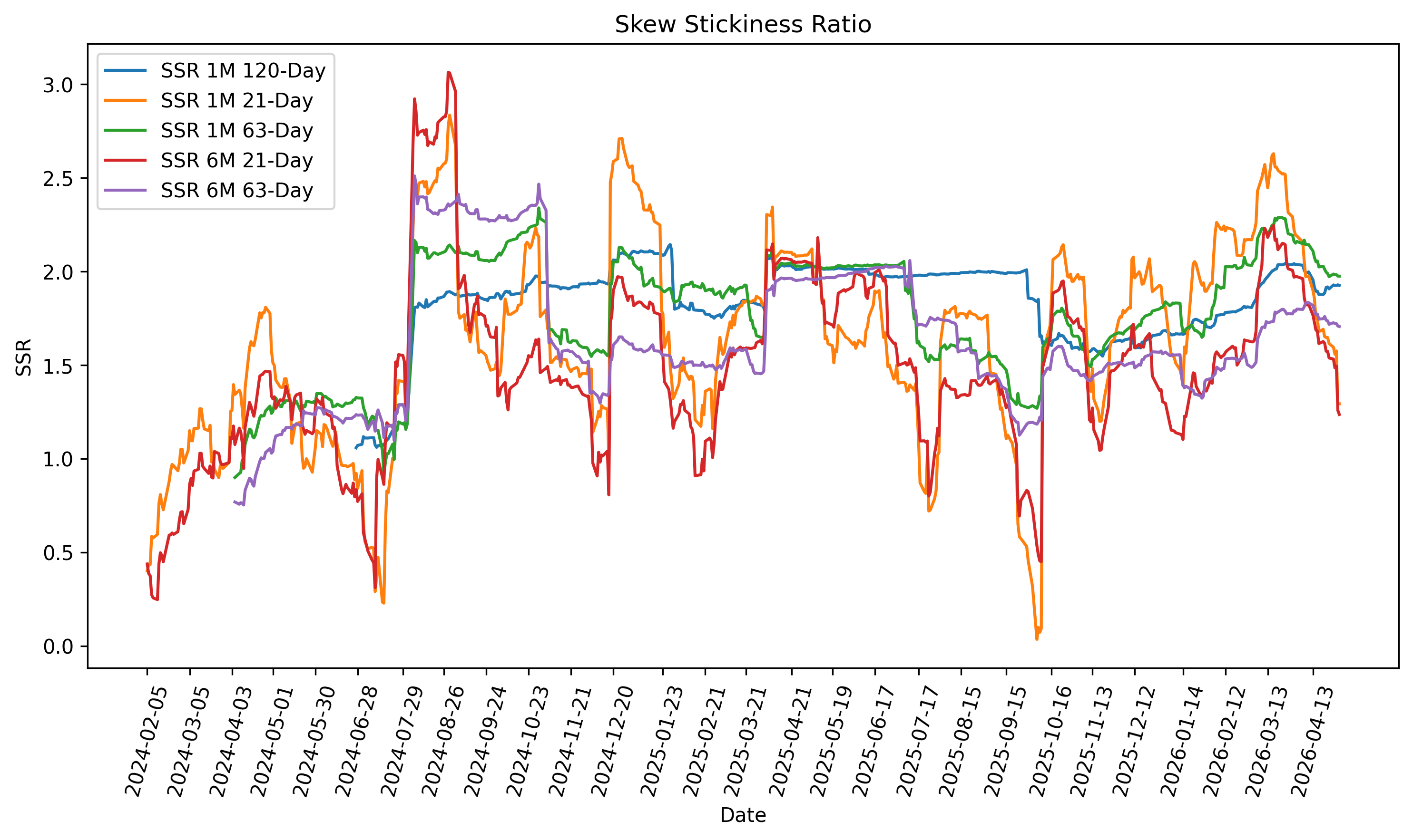
The value of SSR is typically between 1 and 2 and 1.5 on average for equities but as with any realized calculation it is an estimate and can get messy so that is why we see values jump above 2.

Implied SSR:

Where \(\mathcal{S}_{t,T}\) and \(\psi(T)\) are representations of the ATM skew. Both above formulas are the same. The implied SSR is calculated from model parameters so its formulation can be model dependent. We can use the SSR derived from some model to actually test how well the model describes market dynamics. Some volatility models have an amazing fit for the surface but their SSR is completely off, this is the case for Local vol models where we get an exact surface fit, but an SSR of 2 which isnt an accurate description of spot vol dynamics. The only analytically tractable implied SSR I could find is from the 2-factor Bergomi model, which makes sense because he literally created the SSR, but I show the formula below:

\[R(T) = \frac{ \displaystyle\sum_i w_i \rho_i \, \frac{1-e^{-k_iT}}{k_iT} }{ \displaystyle\sum_i w_i \rho_i \, \frac{k_iT-\left(1-e^{-k_iT}\right)}{(k_iT)^2} }\]

Conclusion

In this post I really only scratched the surface (no pun intended) on spot vol dynamics, fixed strike and floating strike vol and the SSR. A lot of the stuff I touched on only measure how spot moves with the ATM IV but what about other parts of the surface? Just like we estimate a beta for the change in ATM IV wrt spot we can estimate how a risk reversal (skew) or butterfly (convexity) change with spot. We can also replace the ATM IV in the SSR with some floating strike vol like 90% moneyness or 25 delta put and calculate the SSR wrt those vols. There is literally a whole surface to explore and modeling how the whole surface changes as spot changes can give vol traders a huge edge. This is something I would like to explore in future posts but I’m sure you’re tired of reading this one so we end it here. I hope you enjoyed and learned something, also if you are a practitioner in the field and want to connect you can find my LinkedIn on the home page of this website, I would love to learn more if there is anything you can introduce to me!

Refrences

References

• Bergomi, L. (2009). Smile Dynamics IV. Société Générale Research.

• Bennett, C. (2014). Trading Volatility. Financial Times Press.

• Derman, E. (2008). Volatility Smile Lecture Series, Columbia University, E4718: Advanced Modeling.

• Gatheral, J. (2023). Computing Skew-Stickiness. Bloomberg Quant Seminar.

• Abi Jaber, E., & Li, S. (2026). Capturing Smile Dynamics with the Quintic Volatility Model: SPX, Skew-Stickiness Ratio and VIX.